Support Vector Machines

Overview

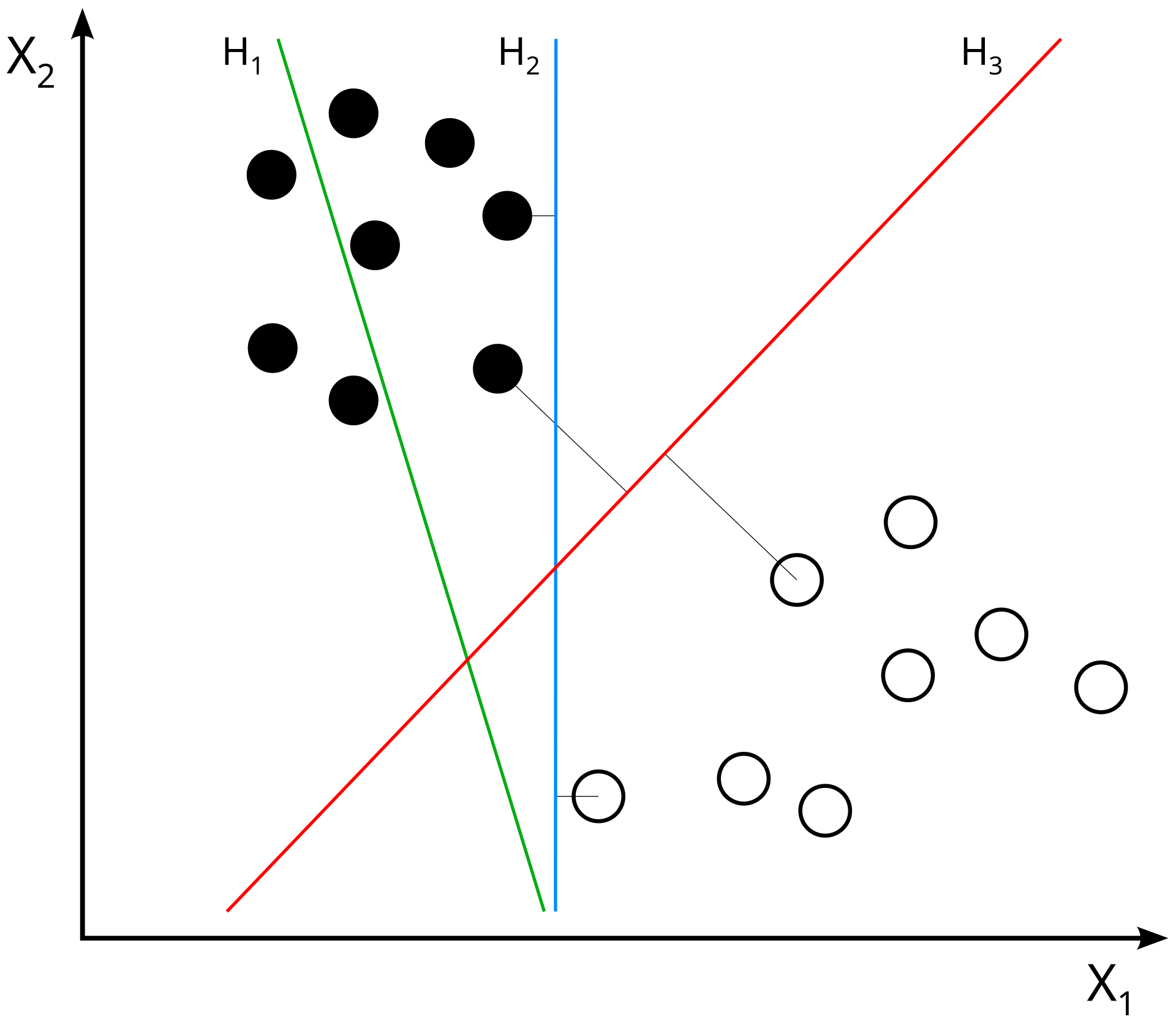
The Support Vector Machine is a supervised machine learning technique that analyzes data for classification and regression analysis. With the application of SVMs, a data point is viewed as a p-dimensional vector with a classification, and we want to be able to separate and classify new data points using a linear separator. The idea is that within infinite dimensions, we would be able to draw a "line" or hyperplane through the points to classify them. Upon finding a linear separator for the data, we aim to maximize the margins between points.

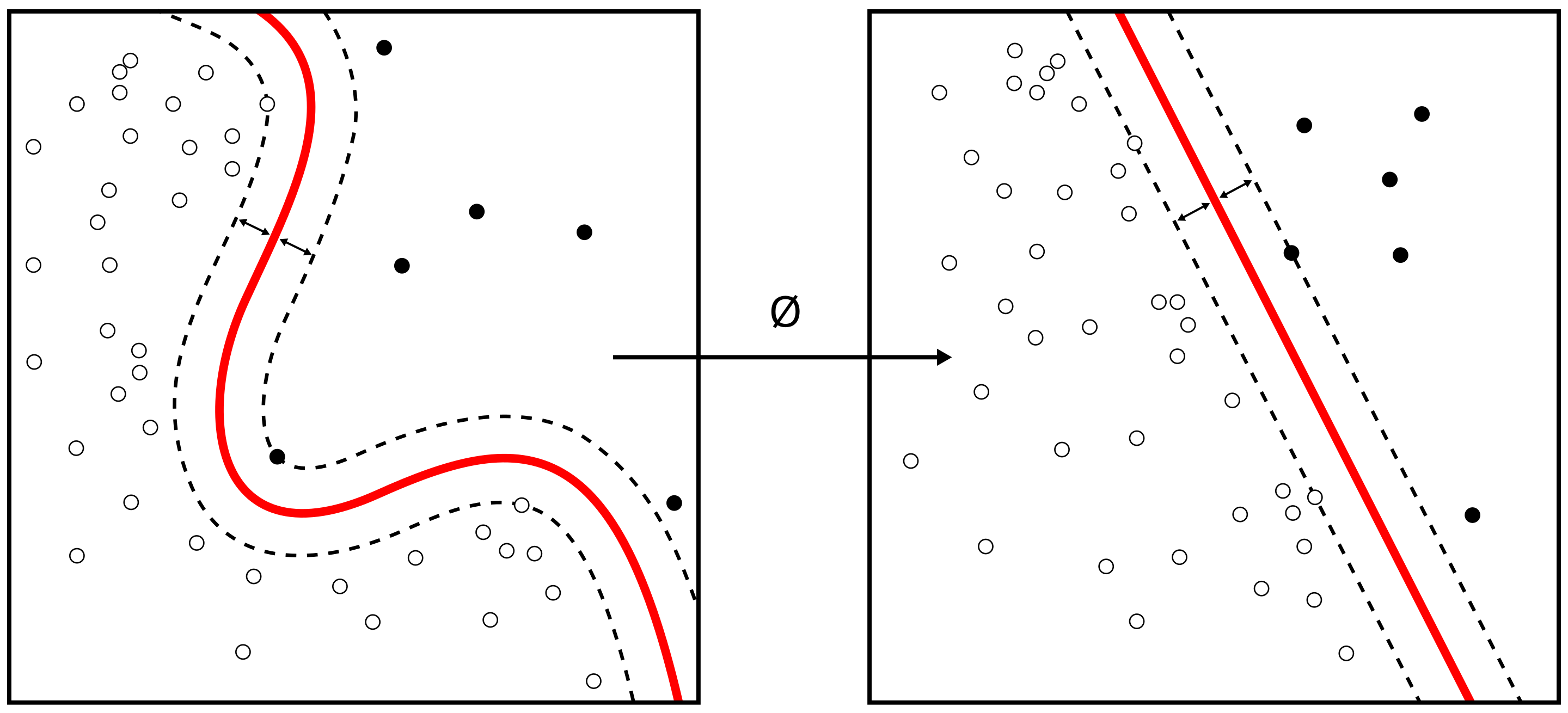
One powerful application of SVM is the kernel trick, which allows us to calculate the inner product between two data points in the transformed space directly, without having to explicitly transform the data into high-dimensional space. This saves us from having to use massive amounts of computing power and enables efficient training. It also allows us to apply and utilize nonlinear kernels to solve more complex problems.

Two examples of useful kernels:

• Polynomial Kernel
  • K(x_i, x_j) = (x_i · x_j + c)^d
  • Where c is a constant and d is the degree of the polynomial
  • Higher dimensions (d > 2) represent more complex relationships, but they may lead to overfitting.
• Radial Basis Function (RBF) Kernel
• K(x_i, x_j) = exp(-γ||x_i - x_j||²)
• Where γ is a hyperparameter that determines the influence of a single training example.
• γ is inversely proportional to the radius of influence of the support vectors.

Polynomial Kernel Example (mapping a 2d point):

We are using a polynomial kernel with parameters \( r = 1 \) and \( d = 2 \) to "cast" a 2D point \( x = [x_1, x_2] \) into a higher-dimensional space. The polynomial kernel formula is:

\( K(x, y) = (x \cdot y + r)^d \)

Step 1: Polynomial Expansion

For a 2D point \( x = [x_1, x_2] \), expanding the formula \( (x_1 \cdot y_1 + x_2 \cdot y_2 + 1)^2 \) gives:

\( (x_1^2, x_2^2, \sqrt{2}x_1x_2, \sqrt{2}x_1, \sqrt{2}x_2, 1) \)

This is the higher-dimensional feature space where the kernel "maps" the original 2D point.

Step 2: Example Point

Let’s take a specific example: \( x = [2, 3] \).

• \( x_1^2 = 2^2 = 4 \)
• \( x_2^2 = 3^2 = 9 \)
• \( \sqrt{2}x_1x_2 = \sqrt{2} \cdot 2 \cdot 3 = 6\sqrt{2} \)
• \( \sqrt{2}x_1 = \sqrt{2} \cdot 2 = 2\sqrt{2} \)
• \( \sqrt{2}x_2 = \sqrt{2} \cdot 3 = 3\sqrt{2} \)
• \( 1 = 1 \) (constant term)

Step 3: Final Transformed Point

The transformed point in the higher-dimensional space is:

\( \phi([2, 3]) = [4, 9, 6\sqrt{2}, 2\sqrt{2}, 3\sqrt{2}, 1] \)

Using the polynomial kernel, the original 2D point \( [2, 3] \) has been "cast" into a 6-dimensional space. Each term corresponds to a feature created by expanding the kernel formula.

Data Prep

Supervised models require labeled data. In this case, we use snow-water equivalent measures to create a binary label for snow. We will use this for our classification problem.

In the code above, we split the data into train/test splits. Included is an output of the data as well. Training and test datasets must be disjoint. We are attempting to train a model, and then test on unseen data to evaluate the model accuracy.

Lastly, data must be numeric for this model. The reason is because the model is a computation. Nulls and categorical data such as text will cause the model to simply error out due to not being able to complete the computation.

Code

Results

Results are mixed - all three kernels (with three different cost functions) tend to perform well with little difference between the results. When looking at the decision boundary graphs, we observe the difference in approach between linear, polynomial, and RBF.

Conclusions

Using a support vector machine approach for snow, we will then attempt to apply the model prediction to both RCP 4.5 and 8.5 (moderate and severe climate projections). We will also attempt to perform a time-series model for 8ft depth soil moisture. These two modeled features will feed into our ultimate streamflow prediction within the final neural network and ensemble sections.