Clustering

Overview

In this analysis, we have applied three different clustering methods: KMeans, Dendrogram (Hierarchical Clustering), and HDBSCAN. Each method has its own strengths and weaknesses, and they can provide different insights into the data. Below, we compare and contrast the results of these clustering methods.

1. KMeans Clustering

• Strengths:
  • Simplicity and Speed: KMeans is simple to implement and computationally efficient, making it suitable for large datasets.
  • Predefined Number of Clusters: It allows the user to specify the number of clusters, which can be useful if the expected number of clusters is known.
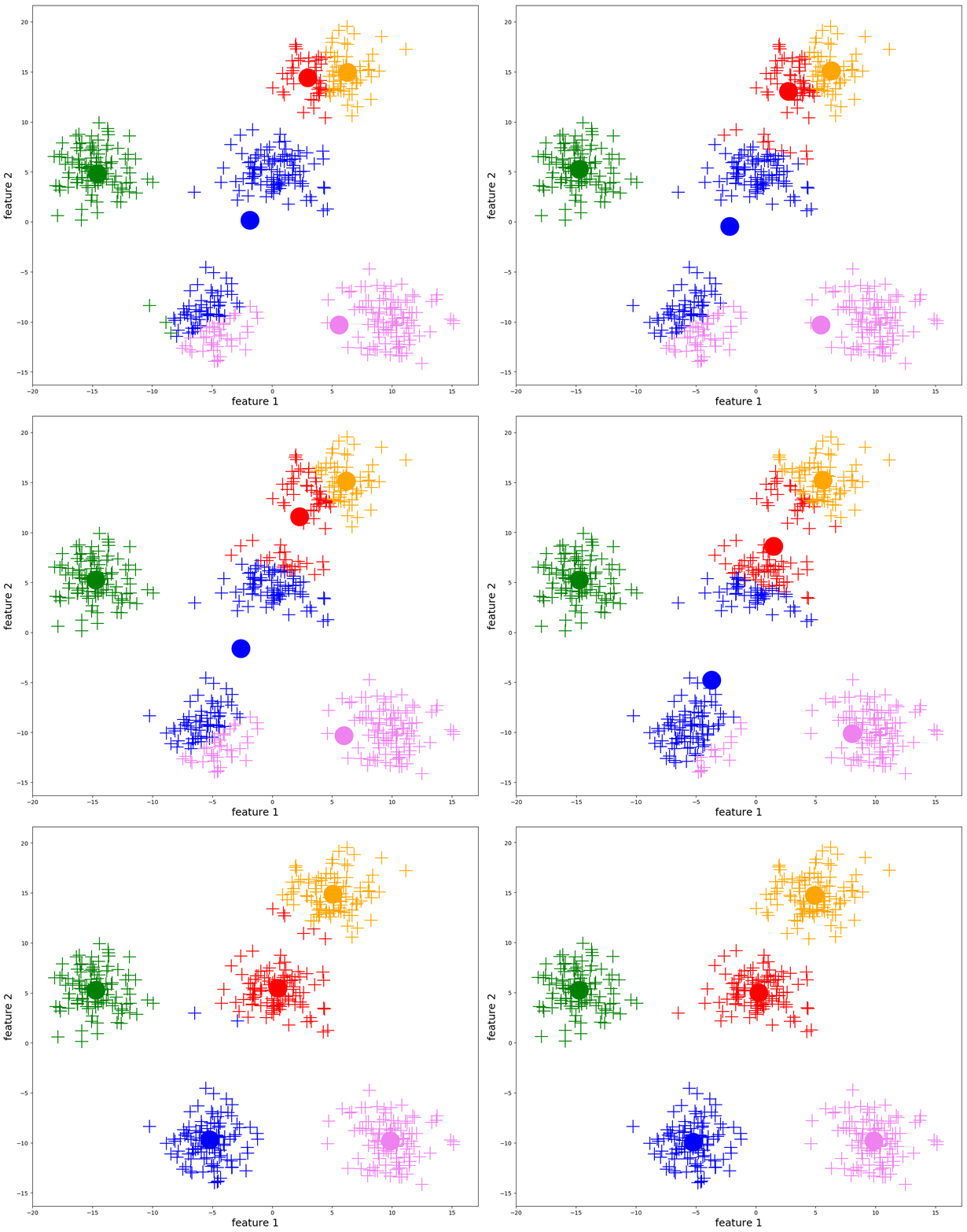
  • Euclidean Distance: KMeans typically uses Euclidean distance as a metric to assign points to the nearest centroid, which works well for spherical clusters. The analysis below will utilize Euclidean distance.
• Weaknesses:
  • Assumption of Spherical Clusters: KMeans assumes that clusters are spherical and equally sized, which may not be true for all datasets.
  • Sensitivity to Initial Centroids: The algorithm can converge to different solutions based on the initial placement of centroids, making it sensitive to initialization.
  • Poor Noise Handling: KMeans does not handle noise and outliers well, as it assigns every point to a cluster.
  • Limitations of Euclidean Distance: When clusters are not spherical or contain outliers, Euclidean distance may not perform well, leading to poor cluster assignment.

2. Dendrogram (Hierarchical Clustering)

• Strengths:
  • Hierarchical Structure: Dendrogram provides a hierarchical view of the data, allowing the user to visualize the merging process of clusters.
  • No Need for Predefined Number of Clusters: The method does not require the number of clusters to be specified initially. Instead, a threshold can be set to cut the dendrogram at the desired level.
  • Flexible Distance Metrics: Hierarchical clustering can use various distance metrics such as Euclidean, Manhattan, or Cosine similarity, making it adaptable to different types of data. For this analysis, we use the default Euclidean distance.
• Weaknesses:
  • Computational Complexity: Hierarchical clustering can be computationally expensive, especially for large datasets.
  • Choice of Threshold: The final clusters depend on the choice of the threshold used to cut the dendrogram, which can be subjective.
  • Scalability Issues: Hierarchical clustering may not scale well to very large datasets when complex distance metrics are used.

3. HDBSCAN (Hierarchical Density-Based Spatial Clustering of Applications with Noise)

• Strengths:
  • Density-Based Clustering: HDBSCAN is capable of finding clusters of varying densities, making it suitable for data with clusters of different shapes and sizes.
  • Noise Handling: It effectively identifies and handles noise points, which are not assigned to any cluster.
  • No Need for Predefined Number of Clusters: Unlike KMeans, HDBSCAN does not require the number of clusters to be specified beforehand.
  • Flexible Distance Metrics: HDBSCAN can work with a variety of distance metrics, including Euclidean, Manhattan, and Cosine similarity, which allows it to adapt to different types of data distributions. We will use the default Euclidean distance.
• Weaknesses:
  • Parameter Sensitivity: The results can be sensitive to the choice of parameters such as min_samples and min_cluster_size.
  • Computational Complexity: HDBSCAN can be computationally intensive for large datasets.

KMeans

KMeans - Temperature, Precipitation, and Snow Water Equivalent 3D Plot

Note that cluster centroids are viewable, you just need to zoom in a bit.

Hierarchical

Density-based

Conclusion

Each clustering method offers unique insights and has its own advantages and limitations. KMeans is efficient for large datasets with a known number of clusters. Based on the centroid-distance calculation process, we get 4 distinct clusters in our results that roughly translate to seasons. Dendrogram provides a hierarchical perspective. Based on the agglomerative clustering we see 4 distinct groupings of the columns of the streamflow prediction dataset. Generally, soil moisture is grouped together, precipitation and temperature is grouped together, and snow water equivalent is grouped together. This serves as a useful validation to ensure like-behaving values. HDBSCAN is suitable for data with varying densities and noise. We chose a comparison between temperature and precipitation to try and uncover clustered data. In general, HDBSCAN does a good job at identifying a gradient of like-behaving data. This may not correspond to seasons as strictly as KMeans, but it does indicate a more granular look at how temperature and precipitation interact.